De Novo Assembly using NGS data
De Novo Assembly
De Novo Assembly is the art of creating reference genomes from scattered data.
This walkthrough follows the steps of the assembly process found in this recently published paper (with me as a co-first author): “The survey and reference assisted assembly of the Octopus vulgaris genome” DOI: 10.1038/s41597-019-0017-6.
Basic Terms
First some basic terms to understand the process:
- Reads: This is the raw data (from the sequencer).
- Unitigs: These are combined reads, up to the point were a possible variation is available (are extended, corrected reads)
- Contigs: These are combined unitigs, where a dessition is made for the variant position.
- Scaffolds: These are combined contigs, the contigs are linked together (information is in the reads), but how they are linked is missing. So contigs are combined together, with a number of Ns in between.
- Chromosomes: These are combined scaffolds, this is always the wanted level to finish the project, however in most cases, this level is unable to reach.
In order to get a correct and representable draft reference genome, it is important to begin with a decent sequencing depth. For NGS data this would be a 60-80x coverage. To estimate the number of needed reads, this can be calculated using various databases on the estimated genome size. Besides this, it is recommended to use long reads (for instance Illumina Pair end 250bp).
Read Quality Control
First do some basic QC:
fastqc -o fastqc -t 20 -d raw raw.R1.fastq.gz raw.R2.fastq.gz
If you see something strange here, do some trimming.
Pre-Computations:
Now it is time to discover the data, and get an idea on how big the genome is (based on the sequenced data), and how complex.
sga preprocess -p 1 raw.R1.fastq raw.R2.fastq > sga_preprocess/sga_readfile.fastq 2> sga_preprocess/sga_preprocess.log;
sga index -a ropebwt --no-reverse -t 4 sga_preprocess/sga_readfile.fastq > sga_preprocess/sga_index.log;

sga preqc -t 4 --force-EM sga_preprocess/sga_readfile.fastq > sga_preqc/raw.preqc;
sga-preqc-report.py sga_preqc/raw.preqc sga/src/examples/*.preqc
This generates an interesting pdf report. I will highlight some of the most interesting graphs below. It is always interesting to create 2 versions of the report: one only containing your data, and one containing the examples. This way you will have a clear graph of only your data, but also the possibility to compare your data to the known other example genomes. Each genome included in the example data has special fetures (like the oyster, which contains a lot of repeats).
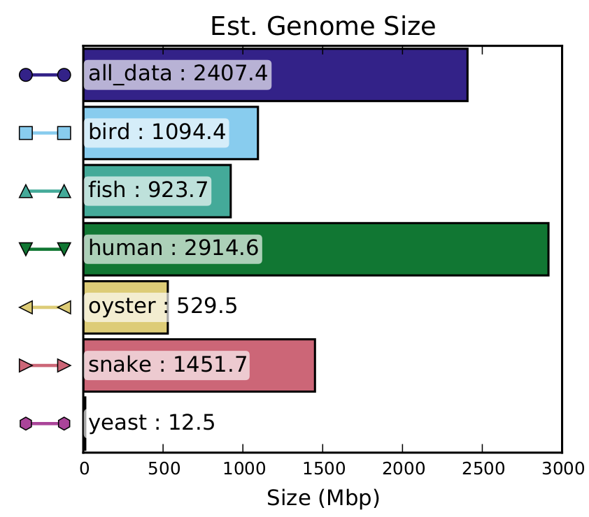
Estimated Genome Size
This graph shows the estimated genome size found in the raw data. Beware that if the genome contains a lot of big repeat regions (larger that the sequencing length), these will be merged to the sequencing length in this graph. Otherwise if the genome has a high number of variations, the alleles will not be merged, resulting in counting twice the length of these alleles.
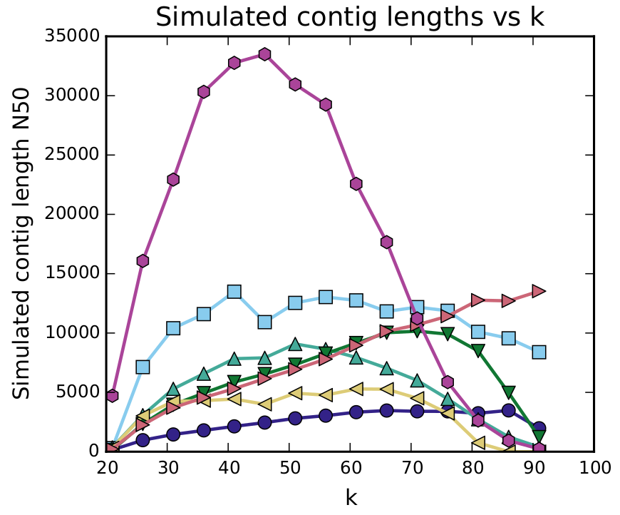
Simulated Contig Length
This graph shows a simulation on the contig length, using different kmers. The ideal kmer to pick for your assembly is at the peak of the graph. If this graph has multiple peaks, you can try multiple kmers, and compare these assemblies.
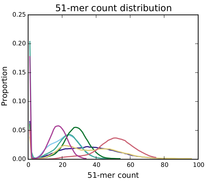
Kmer Count Distribution
This graph shows a distribution of the proportion of fragments of a 51-mer count. If you only see one peak, your genome does have a high number of variants. If you see 2 peaks (the graph can also be a smear, see the light blue and yellow lines on the graph), this indicates a lot of variants. The first peak is the homozygous peak, the second the heterozygous peak. How higher the first peak the more 51mers are containing a variant. The place of the second peak will be equal to the sequencing depth of the genome. A smaller peak further in the data indicates big repeat regions.
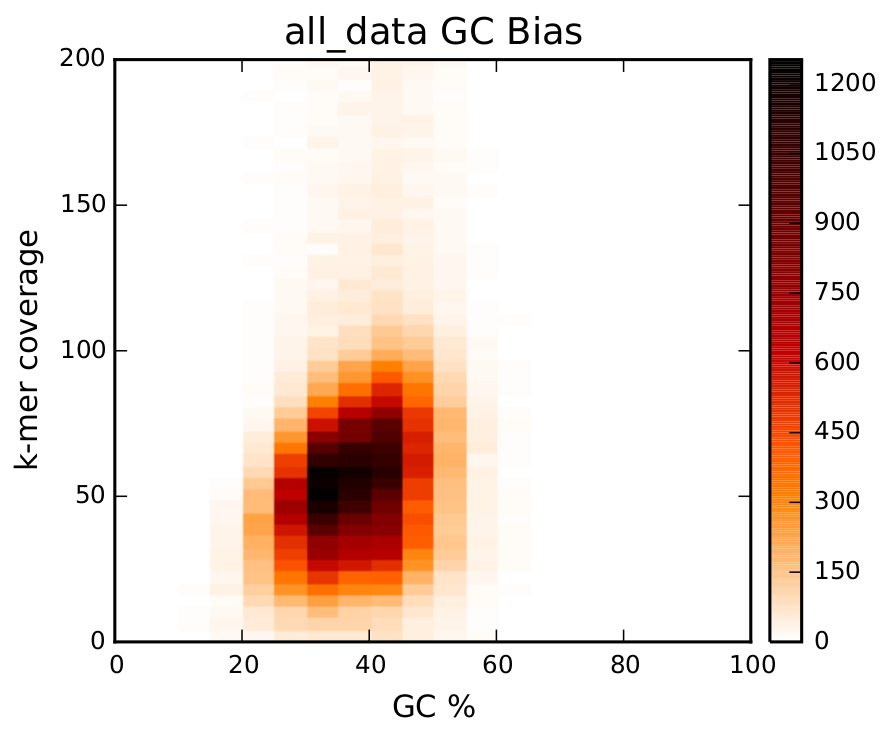
GC Bias
This graph shows a distribution of the GC Bias. On the x axis, you see the percentage of GC in your genome. If the percentage is to much to the left or right, it is possible that, due to the sequencer limits, parts of your genome is not sequenced. A smear on top of the graph (like here), indicates long repeat regions.
Assembly
There are a lot of different assembly tools available. All have there PRO and CONS. I like to use ABySS, since it is a easy to use, frequently updated tool. It uses de Bruiyn graphs. A good idea is always to use multiple assemblers (and different methods, like string graph), and compare the assemblies.
#using ABySS/2.0.2

cd abyss_41
abyss-pe name="octopus" k=41 lib="pe700" pe700="raw.R1.fastq.gz raw.R2.fastq.gz" np=50 j=50;

#with:
#name: the name of the result assembly
#k: the selected kmer
#lib: the name of the library
#pe700: are the files of the given library
#np: number of processors
#j: number of jobs it can execute automatically
The important output files are:
- octopus_abyss41_k41-contigs.fa
- octopus_abyss41_k41-scaffolds.fa
Optional Check
You can optionally check how well this assembly is, by mapping the raw data to the created reference. Check how many data mapped uniquely, and how many data multiple times. If the number of multimappings is high, the genome has a lot of mutations, the graph couldn’t handle, and a reduction is needed.
Reduction of Scaffolds
Redundans compares the smaller contigs/scaffolds to the larger ones, and tries to merge these (if they are of the same allele). After this merge, a new scaffolding step is performed.
#using redundans/v0.13c
redundans -t 40 -v -i raw.R1.fastq raw.R2.fastq -f abyss_41/octopus-contigs.fa -o redundans;
The important output files are:
- contigs.fa
- scaffolds.fa
Reference Assisted Scaffolding
If a reference of a close related species is available, this can be used to scaffold this genome. In this process the scaffolds are compared to the other reference genome (using blast), overlapping fragments are merged, others are scaffolded in order to get a completer draft genome.
#using BLAST/2.8.0-alpha

#create a blast database of the other genome (here in $BLAST_GENOME)
blastn -query redundans/output/scaffolds.fa -out blast/octopus.blast.out -db $BLAST_GENOME -evalue 0.00001 -perc_identity 80 -max_hsps 2 -outfmt 6 -db_hard_mask 30 -word_size 50

#using chromosomer/0.1.3
cd chromosomer
chromosomer fastalength redundans/output/scaffolds.fasta chromosomer.fastalength

chromosomer fragmentmap -r 1.2 blast/octopus.blast.out 800 chromosomer.fastalength chromosomer.fragmentmap
#-r is ratio: can be between 1 and 2
#800 is the gapsize

chromosomer fragmentmapstat chromosomer.fragmentmap chromosomer.fragmentmap.stats

chromosomer assemble chromosomer.fragmentmap redundans/output/scaffolds.fasta chromosomer_scaffolds.fasta

#combine all files to complete genome
cp chromosomer_scaffolds.fasta complete_genome.fasta
awk 'BEGIN{}{if(FNR==NR){arr[$1]="in"}else{if($1~">"){tp=0; name=substr($1,2); if(name in arr){tp=1;}}}if(tp==1){print $0;}}' chromosomer_unplaced.txt $CONTIG_FILE >> complete_genome.fasta
awk 'BEGIN{}{if(FNR==NR){arr[$1]="in"}else{if($1~">"){tp=0; name=substr($1,2); if(name in arr){tp=1;}}}if(tp==1){print $0;}}' chromosomer_unlocalized.txt $CONTIG_FILE >> complete_genome.fasta
As a result a new genome is created, and can be found in complete_genome.fasta
Assesment of the genome
The quality of the genome can be checked by creating a report using quast. This report contains different quality massures like N50, L50, number of Ns, …
#using QUAST/4.3

quast.py -t 20 -o quast chromosomer/complete_genome.fasta
BUSCO assesment
Busco checks the created genome for known concerved genes. If you find a high number of highly concerved genes, you will have created a good draft genome.
#using busco/3.0.2

busco -i genome.fa -l busco/3.0.2/lineage/metazoa_odb9 -o final_genome -m genome -c 36
#-l is the database of busco genes, please select the most approrpiate one
Further adjustments
You can mask repeat regions:
#using BLAST/2.8.0-alpha

windowmasker -in genome.fa -infmt fasta -mk_counts -parse_seqids -out genome.counts -sformat obinary
windowmasker -in genome.fa -infmt fasta -ustat genome.counts -outfmt maskinfo_asn1_bin -out genome.asnb
windowmasker -in genome.fa -infmt fasta -ustat genome.counts -outfmt fasta -out genome_masked.fa